Exploring Semantic Similarity in 3D with CLIP and t-SNE#

In this post, I dive into the fascinating world of word embeddings and semantic similarity visualization. Using OpenAI’s powerful CLIP model and dimensionality reduction techniques like t-SNE, I create an interactive 3D scatter plot that reveals the relationships between words based on their meanings.

Background and Inspiration#

The inspiration for this project came from an interesting encounter with the word “virile” in the context of Stable Diffusion models. When I first came across model series like “Virile Reality” and “Virile Stallion,” I had never seen the word “virile” before. I initially read it in my head as “vee-rill” or “vai-raisle” instead of the correct pronunciation “vur-uhl” or “veer-uhl.” This piqued my curiosity about the semantic similarity of virile-adjacent words in CLIP, the text encoder used by Stable Diffusion models.

As a side note, Virile Reality (SD1.5 checkpoint) and Virile Stallion (SDXL checkpoint, Pony Diffusion V6 based) are both exceptional models created by @Scratchproof on the Unstable Diffusion Discord server. These models genuinely excel in the areas of inclusivity in AI by combating the incredibly serious and disgusting gender bias against men in AI training data, which manifests as a lack of understanding of critical aspects of our world by diffusion models.

A Side Note on Alignment#

Giving these models a skewed version of our world inherently makes them flawed and will always cause unforeseen issues. Censoring a model, whether it’s an LLM, diffusion, auto-regression, or whatever, effectively lobotomizes its understanding, regardless of what is censored.

It’s like locking a toddler in a basement, lying to them about the world for their entire life, and then wondering why they didn’t grow up into a well-rounded adult. Although this analogy may seem extreme, it effectively illustrates the consequences of censorship and bias in AI training data. It’s quite obvious in hindsight, but it still plagues research efforts.

Perhaps the most infamous and recent example is the Stable Diffusion model, SD3 medium (2B parameter variant with an abysmal license), which consistently fails to produce human anatomy due to heavy censoring in the pre-training stage (sanitizing training data). This censorship ruined the model even before the post-training alignment efforts, which also effectively make the model useless in other areas as well.

Explanation of the Visualization#

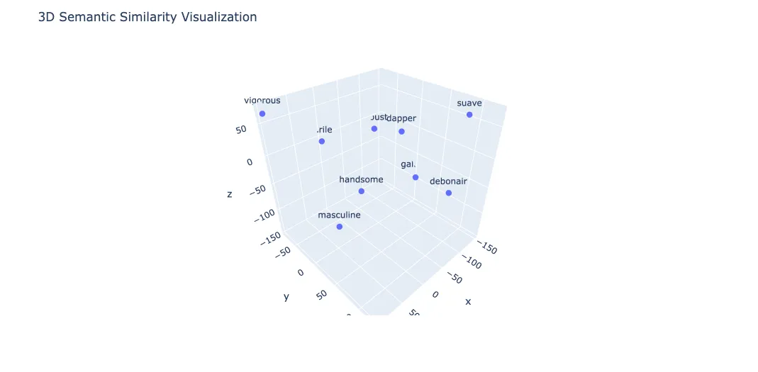
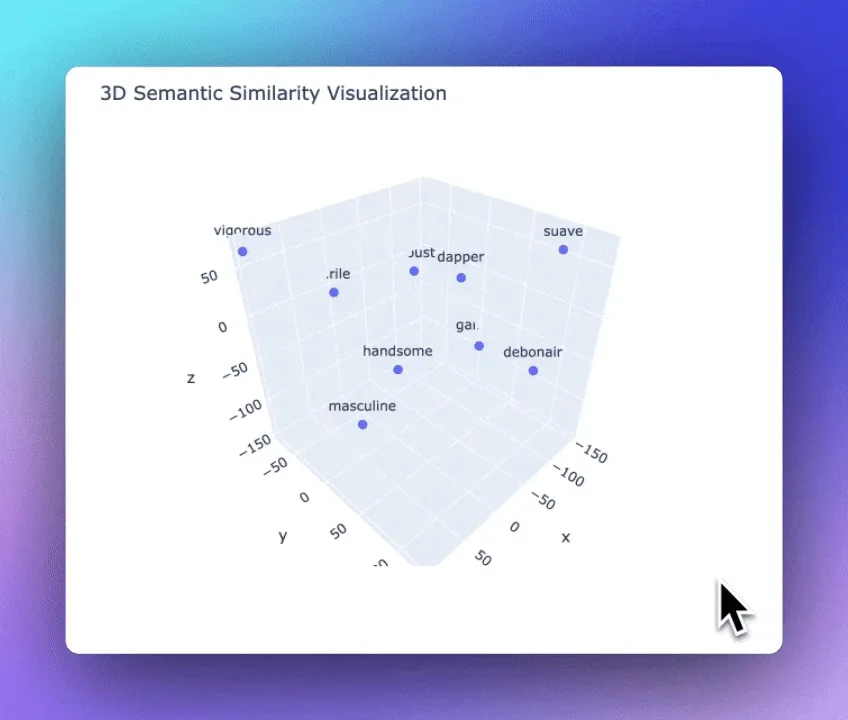
What You’re Looking At:#

• 3D Scatter Plot: Each point represents a word, with positions derived from high-dimensional vectors capturing the words’ meanings.
• CLIP Model: A neural network from OpenAI that understands text and images, providing embeddings (vectors) for words.

Key Concepts:#

1. Word Embeddings: These are vectors that represent the meaning of words based on their usage in large datasets.
2. t-SNE: A method to reduce the complexity of high-dimensional vectors so they can be visualized in 3D, preserving their relationships.

Interpretation:#

• Proximity: Words close together have similar meanings. For example, “virile” and “vigorous” are near each other, indicating similar meanings.
• Clusters: Groups of words like “handsome,” “gallant,” and “masculine” cluster together, showing they share related meanings.

How I Created the Plot:#

1. Using CLIP: I used the CLIP model to get embeddings for my words. These embeddings are high-dimensional vectors representing word meanings.
2. Finding Similar Words: I started with a list of words I thought were related to “virile.” I asked ChatGPT to refine it and add similar words based on meaning and “fanciness.”
3. Dimensionality Reduction with t-SNE: I used t-SNE to reduce these high-dimensional vectors to 3D for visualization.
4. Plotting with Plotly: I used Plotly to create the interactive 3D scatter plot. You can rotate and zoom to explore the relationships between the words.

Code Walkthrough#

Here’s a breakdown of the Python code I used to create this visualization:

import torch
from transformers import CLIPTokenizer, CLIPModel
import plotly.express as px
from sklearn.manifold import TSNE
import pandas as pd

# Load the CLIP model and tokenizer
model_name = "openai/clip-vit-base-patch32"
model = CLIPModel.from_pretrained(model_name)
tokenizer = CLIPTokenizer.from_pretrained(model_name)

First, I load the CLIP model and tokenizer from the Transformers library. CLIP is a powerful model that understands both text and images.

# Define the target word and related words
target_word = 'virile'
related_words = ['handsome', 'dapper', 'suave', 'debonair', 'masculine', 'gallant', 'vigorous', 'robust']

words = [target_word] + related_words
inputs = tokenizer(words, return_tensors="pt", padding=True)

# Get the embeddings for the words
with torch.no_grad():
    embeddings = model.get_text_features(**inputs)

I define the target word “virile” and a list of related words. I tokenize these words and pass them through the CLIP model to get their embeddings.

# Reduce dimensions to 3D with adjusted perplexity
tsne = TSNE(n_components=3, random_state=0, perplexity=5)
embeddings_3d = tsne.fit_transform(embeddings)

Using t-SNE, I reduce the high-dimensional embeddings to 3D for visualization. The perplexity parameter is adjusted to handle the small number of words.

# Prepare data for Plotly
df = pd.DataFrame(embeddings_3d, columns=['x', 'y', 'z'])
df['word'] = words

# Plot the words
fig = px.scatter_3d(df, x='x', y='y', z='z', text='word')

fig.update_traces(marker=dict(size=5), selector=dict(mode='markers+text'))
fig.update_layout(title='3D Semantic Similarity Visualization', scene=dict(aspectmode='cube'))

fig.show()

Finally, I create a DataFrame with the 3D coordinates and the corresponding words. Using Plotly Express, I plot the words as points in an interactive 3D scatter plot.

You can find the full code in this Colab notebook.

Additional Notes#

To find similar words dynamically, I would need to precompute embeddings for a large dictionary. This would allow for quick comparisons to find the closest matches to any given word.

Exploring semantic similarity using advanced AI models like CLIP opens up exciting possibilities for understanding and visualizing the relationships between words. I hope this post has given you a glimpse into the power of combining cutting-edge NLP techniques with interactive data visualization.

Stay tuned for more adventures in AI and data science!

Mark June 2024